Guaranteed Higher Grade!
Free Quote

There were 46 crude oil spills of at least 1000 barrels from tankers in U.S. waters during 1974–1999. The website for this book contains the following data: the number of spills in the ith year, Ni; the estimated amount of oil shipped through US waters as part of US import/export operations in the ith year, adjusted for spillage in international or foreign waters, bi1; and the amount of oil shipped through U.S. waters during domestic shipments in the ith year, bi2. The data are adapted from [11]. Oil shipment amounts are measured in billions of barrels (Bbbl). The volume of oil shipped is a measure of exposure to spill risk. Suppose we use the Poisson process assumption given by Ni|bi1, bi2 ∼ Poisson(λi) where λi = α1bi1 + α2bi2. The parameters of this model are α1 and α2, which represent the rate of spill occurrence per Bbbl oil shipped during import/export and domestic shipments, respectively
a. Derive the Newton–Raphson update for finding the MLEs of α1 and α2.
b. Derive the Fisher scoring update for finding the MLEs of α1 and α2.
c. Implement the Newton– Raphson and Fisher scoring methods for this problem, provide the MLEs, and compare the implementation ease and performance of the two methods.
d. Estimate standard errors for the MLEs of α1 and α2. e. Apply the method of steepest ascent. Use step-halving backtracking as necessary.
f. Apply quasi-Newton optimization with the Hessian approximation update given in (2.49). Compare performance with and without step halving.
g. Construct a graph resembling Figure 2.8 that compares the paths taken by methods used in (a)–(f). Choose the plotting region and starting point to best illustrate the features of the algorithms’ performance
 100+ Accounting Dissertation Topics for Students
Narrowing down the right dissertation topic from a broad field like accounting can be a challenging
 100+ Unique Statistics Project Ideas for Students
Statistics is the science of collecting, analyzing, and interpreting data. Whether you’re in high
 Informative Essay Topics - Latest Writing Ideas for Your Paper
Have you found yourself struggling to gather interesting ideas for an informative essay? The pressu
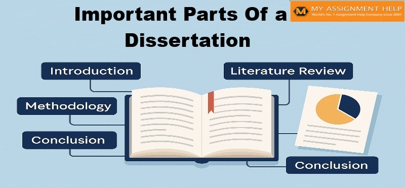 Important Part of Dissertation
Get Writing Help On Every Important Part Of Dissertation. Did you miss an important part of