Quantitative Analysis In Business: A Case Study Essay.

Descriptive Statistics and Graphical Analysis

Quantitative analysis is a basic part of each and every business or industry. In each business and industry, there is a huge amount of data produced and therefore management team of such businesses or industries needs to analyze these data sets for the planning and marketing. Quantitative analysis also called as statistical analysis and it is consist of descriptive statistical measures as well as some inferential measures. Statistical analysis plays an important role in the planning and other functions of managerial team of the business or company or industry. Here, we have to study of quantitative techniques in business for one particular case. We are given a data for sunglasses for 12 months for the variables sales, prices, advertising expenditure, number of households, average sales experience and mean daily hours. The detailed table including the data is given in the appendix. Also, units for each variable are explained detail in the table attached in the appendix. We have to analyze this data by using some statistical methods. We have to see some descriptive statistics for the each variable under study. Also we have to see some graphical analysis for the given variables. From these graphs, we have to check whether there is any linear relationship or association observed between the two variables or not. For more detail of the linear relationship or association between the different variables under study, we have to see the correlation analysis. For this purpose, we have to see the correlation matrix which shows the relationship between every two variables. From this correlation analysis, we can check whether the linear relationship is significant or not. Also, we have to see the regression model for the given variables. Regression model helps for further estimation. Regression analysis explains the detailed relationship between and among the variables under study. Let us see all this quantitative or statistical analysis step by step given below.

In this part, we have to see the descriptive statistics and graphical analysis for the given variables. First we have to see some descriptive statistics for the given variables such as sales of the sunglasses, price, advertising expenditure, number of households, average sales experience and mean daily hours. Descriptive statistics consist of the mean, mode, median, standard deviation, variance, minimum, maximum, kurtosis, skewness, etc. For the analysis of given variables, we have to use the SPSS software for analysis purpose. The descriptive statistics for the given variables are given in the following tables.

Descriptive Statistics
	N	Minimum	Sum	Mean	Std. Deviation	Variance
Sales	12	75.00	2273.00	189.4167	83.25804	6931.902
Price	12	2.10	49.50	4.1250	1.60631	2.580
Advert_exp	12	2.00	177.00	14.7500	10.48050	109.841
No._households	12	500.00	7456.00	621.3333	102.51061	10508.424
Avg.Sales.experience	12	10.00	177.00	14.7500	2.95804	8.750
Mean_daily_hours	12	2.00	77.80	6.4833	3.16998	10.049
Valid N (listwise)	12

The average sales for the sunglasses is given as 189.4167(£’000). The standard deviation for sales for the sunglasses is given as 83.25804(£’000). All averages and standard deviations are summaries in the above table. Some other descriptive statistics are given in the following table:

Descriptive Statistics
	N	Range	Maximum	Mean	Skewness		Kurtosis
	Statistic	Statistic	Statistic	Std. Error	Statistic	Std. Error	Statistic	Std. Error
Sales	12	243.00	318.00	24.03453	-.061	.637	-1.368	1.232
Price	12	4.70	6.80	.46370	.626	.637	-1.095	1.232
Advert_exp	12	28.00	30.00	3.02546	.136	.637	-1.768	1.232
No._households	12	270.00	770.00	29.59226	.264	.637	-1.787	1.232
Avg.Sales.experience	12	8.00	18.00	.85391	-.163	.637	-1.468	1.232
Mean_daily_hours	12	9.50	11.50	.91510	.076	.637	-1.232	1.232
Valid N (listwise)	12

For the variables sales of sunglasses and average sales experience, the skewness values are negative, this implies that the distribution is skewed at left side for these two variables. For all other variables, the distribution is positively skewed. All kurtosis values are negative for all variables.

Correlation Analysis

Now, we have to see some graphical analysis for the given variables. By using these graphs, we have to check the linear relationship or association between the two variables. For this purpose, we have to use the scatter diagram. Scatter diagram explains the relationship between the two variables graphically. The scatter diagram for the price and sales of sunglasses is given below:

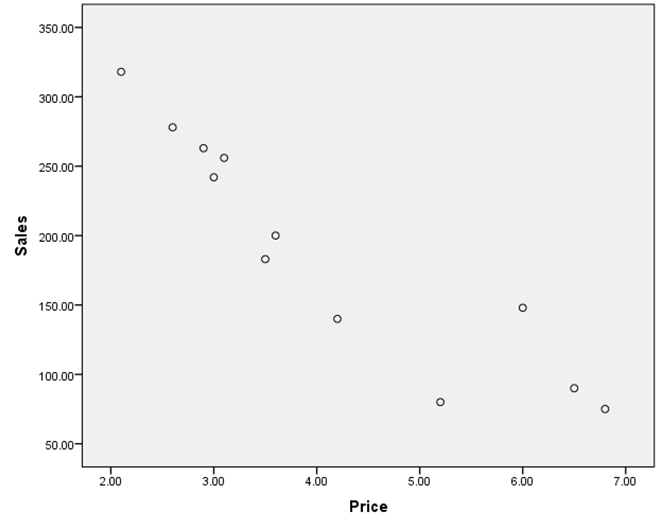
This diagram shows that there is negative association between the two variables sales and price. This scatter plots shows the approximately linear relationship exists between the sales and price. This scatter diagram implies that as the price of the sunglasses increases, the sales of the sunglasses decreases.

Now, let us see the scatter diagram for the variable sales and advertisement expenditure. The diagram is given below:

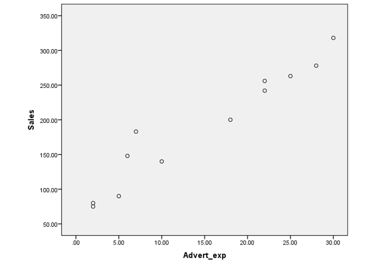
This scatter diagram also shows an approximately linear relationship or correlation between the sales and advertisement expenditure. This scatter shows positive linear relationship exists between the two variables sales and advertisement expenditure of sunglasses. This means that as the advertisement expenditure increases, the sales of the sunglasses also increases.

Now, let us see the scatter diagram for the variable sales and average sales experience for sunglasses. The scatter diagram is given below:

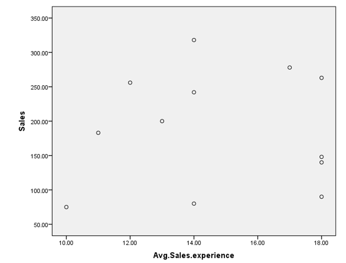
This diagram do not implies any linear relationship or association between the two variables sales of sunglasses and average sales experience for the sunglasses. This implies that the sales of the sunglasses do not depend upon the average sales experience for the sunglasses.

Now, let us see the scatter diagram for the variable sales and number of households for sunglasses. The scatter diagram is given below:

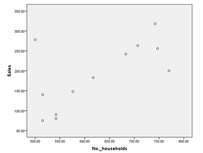
This scatter diagram implies an approximately linear relationship or association exists between the two variables sales of sunglasses and number of household in the area. This scatter diagram represents approximately positive relationship. This means that as the number of household’s increases, the sales of the sunglasses also increases.

Now, let us see the scatter diagram for the variable sales and mean daily hours of sales for sunglasses. The scatter diagram is given below:

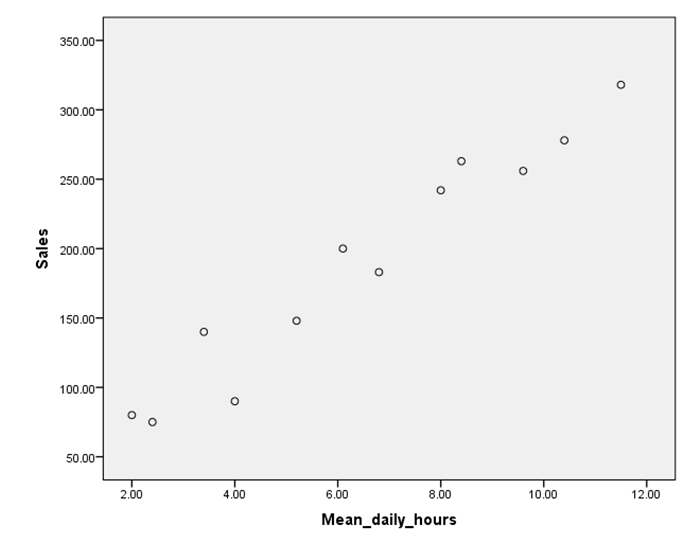
This scatter diagram implies a positive linear relationship exists between the two variables mean daily hours and sales of the sunglasses. This means that as the mean daily hours increases, the sales of the sunglasses also increases.

In the above part, we see the relationship between the two different variables by using the scatter diagram. In this part, we have to find the correlation coefficient between these two different variables under study. Correlation coefficient gives the exact extent of the linear relationship or association between these two variables. For this purpose, we have to find the correlation coefficient between the variables. The SPSS output for the correlation coefficients is given below:

Correlations
		Sales	Price	Advert_exp	No._households	Avg.Sales.experience	Mean_daily_hours
Sales	Pearson Correlation	1	-.922**	.964**	.641*	.049	.973**
	Sig. (2-tailed)		.000	.000	.025	.880	.000
	N	12	12	12	12	12	12
Price	Pearson Correlation	-.922**	1	-.885**	-.601*	.030	-.851**
	Sig. (2-tailed)	.000		.000	.039	.926	.000
	N	12	12	12	12	12	12
Advert_exp	Pearson Correlation	.964**	-.885**	1	.595*	.130	.923**
	Sig. (2-tailed)	.000	.000		.041	.688	.000
	N	12	12	12	12	12	12
No._households	Pearson Correlation	.641*	-.601*	.595*	1	-.272	.586*
	Sig. (2-tailed)	.025	.039	.041		.393	.045
	N	12	12	12	12	12	12
Avg.Sales.experience	Pearson Correlation	.049	.030	.130	-.272	1	.015
	Sig. (2-tailed)	.880	.926	.688	.393		.963
	N	12	12	12	12	12	12
Mean_daily_hours	Pearson Correlation	.973**	-.851**	.923**	.586*	.015	1
	Sig. (2-tailed)	.000	.000	.000	.045	.963
	N	12	12	12	12	12	12
**. Correlation is significant at the 0.01 level (2-tailed).
*. Correlation is significant at the 0.05 level (2-tailed).

From the above table, the correlation between the two variables sales and price is given as     -0.922, and this is high negative relationship. This fact we already observed in the scatter diagram. This correlation coefficient implies that as the price of the sunglasses increases, the sale of the sunglasses decreases and vice-versa. The correlation coefficient between the sales of the sunglasses and advertisement expenditure for the sunglasses is given as 0.964, this implies that there is high positive correlation between the sales of the sunglasses and advertisement expenditure for the sunglasses. This means that if we increase the budget for the advertisement for the sunglasses, it results into the increment of the sales of the sunglasses. The correlation coefficient between the sales of the sunglasses and average sales experience is given as 0.049, this is very low positive correlation coefficient. This implies that there is very low or no any correlation or linear relationship or association exists between the two variables sales of the sunglasses and the average sales experience. This represents that there is no important role for the experience of sales of sunglasses for increasing the total sales for the sunglasses. The correlation coefficient between the sales of the sunglasses and the mean daily hours is given as 0.973 and this is very high positive correlation coefficient. This means that there is strong correlation or linear relationship exists between the two variables sales of the sunglasses and the mean daily hours of sales of sunglasses. If the mean daily hour of sales increases, it results in the total increment of the sales of the sunglasses.

Regression Analysis

In quantitative techniques or statistical analysis, the regression analysis is nothing but the statistical process for the estimating the relationships among the different variables under study. This regression analysis technique includes the formation of regression equation for the estimation purpose. In this technique, we focus on one dependent variable and one or many other independent variables. In the regression analysis, the dependent variable is assumed as the linear function of the one or more than one independent variables. Now, we have to see the regression model for the linear relationship between all these variables. We consider the sales of the sunglasses as the dependent variable and for this regression model, we consider the independent variables as the price of the sunglasses, advertisement expenditure for the sunglasses, number of households in the area, average sales experience and mean daily hours for the sunglasses. The statistical analysis for this regression model for the given variables under study is very important for the future planning for sales of the sunglasses. This model or regression equation will help in planning and management and it will helpful for the estimation purpose. The SPSS output for this regression model is given below:

Descriptive Statistics
	Mean	Std. Deviation	N
Sales	189.4167	83.25804	12
Price	4.1250	1.60631	12
Advert_exp	14.7500	10.48050	12
No._households	621.3333	102.51061	12
Avg.Sales.experience	14.7500	2.95804	12
Mean_daily_hours	6.4833	3.16998	12

Correlations
		Sales	Price	Advert_exp	No._households	Avg.Sales.experience	Mean_daily_hours
Pearson Correlation	Sales	1.000	-.922	.964	.641	.049	.973
	Price	-.922	1.000	-.885	-.601	.030	-.851
	Advert_exp	.964	-.885	1.000	.595	.130	.923
	No._households	.641	-.601	.595	1.000	-.272	.586
	Avg.Sales.experience	.049	.030	.130	-.272	1.000	.015
	Mean_daily_hours	.973	-.851	.923	.586	.015	1.000
Sig. (1-tailed)	Sales		.000	.000	.012	.440	.000
	Price	.000		.000	.019	.463	.000
	Advert_exp	.000	.000		.021	.344	.000
	No._households	.012	.019	.021		.196	.023
	Avg.Sales.experience	.440	.463	.344	.196		.482
	Mean_daily_hours	.000	.000	.000	.023	.482
N	Sales	12	12	12	12	12	12
	Price	12	12	12	12	12	12
	Advert_exp	12	12	12	12	12	12
	No._households	12	12	12	12	12	12
	Avg.Sales.experience	12	12	12	12	12	12
	Mean_daily_hours	12	12	12	12	12	12

Variables Entered/Removeda
Model	Variables Entered	Variables Removed	Method
1	Mean_daily_hours, Avg.Sales.experience, No._households, Price, Advert_expb	.	Enter

a. Dependent Variable: Sales

b. All requested variables entered

The model summary for this regression model is given below:

Model Summary
Model	R	R Square	Adjusted R Square	Std. Error of the Estimate
1	.995a	.990	.982	11.07901

 a. Predictors: (Constant), Mean_daily_hours, Avg.Sales.experience, No._households, Price, Advert_exp

For this regression model, the multiple correlation coefficient R is given as 0.995 and this implies that there is high linear relationship exists between the dependent variable sales of the sunglasses and other independent variables such as price, advertisement experience, number of households, average sales experience and mean daily hours for the sale of sunglasses. The value of coefficient of determination or R square is given as 0.990, this implies that about 99% of the variation in the dependent variable sales of the sunglasses is explained by the independent variables price, advertisement expenditure, number of households, average sales experience and mean daily hours for the sale of sunglasses.

In every regression model, ANOVA is very important for taking decision about the regression model. The ANOVA table is given as below:

ANOVAa
Model		Sum of Squares	df	Mean Square	F	Sig.
1	Regression	75514.449	5	15102.890	123.043	.000b
	Residual	736.467	6	122.745
	Total	76250.917	11

a Dependent Variable: Sales.

b. Predictors: (Constant), Mean_daily_hours, Avg.Sales.experience, No._households, Price, Advert_exp

For this ANOVA table, we get the test statistic value F as 123.043 and the p-value is given as the 0.000. So, here, p-value is less than the level of significance or alpha value 0.05 or 0.01, so we reject the null hypothesis that the given regression model is significant.

The coefficients for the regression equation or model are given in the following table:

Coefficientsa
Model		Unstandardized Coefficients		Standardized Coefficients	t	Sig.	95.0% Confidence Interval for B
		B	Std. Error	Beta			Lower Bound	Upper Bound
1	(Constant)	76.051	46.882		1.622	.156	-38.667	190.768
	Price	-12.114	4.742	-.234	-2.555	.043	-23.718	-.511
	Advert_exp	1.916	1.061	.241	1.806	.121	-.680	4.513
	No._households	.054	.045	.066	1.189	.279	-.057	.164
	Avg.Sales.experience	.981	1.342	.035	.731	.492	-2.302	4.265
	Mean_daily_hours	13.449	2.864	.512	4.696	.003	6.442	20.457
a. Dependent Variable: Sales

The regression equation for this regression model under study is given as below:

Sales = 76.051 – 12.114*Price + 1.916*advertisement expenditure + 0.054*number of households + 0.981*average sales experience + 13.449*mean daily hours.

Conclusion and recommendation (s)

• The correlation between the two variables sales and price is given as -0.922, and this is high negative relationship. This correlation coefficient implies that as the price of the sunglasses increases, the sale of the sunglasses decreases and vice-versa. So, it is recommended that do not increase the price of the sunglasses in high extent.
• The correlation coefficient between the sales of the sunglasses and advertisement expenditure for the sunglasses is given as 0.964, this implies that there is high positive correlation between the sales of the sunglasses and advertisement expenditure for the sunglasses. This means that if we increase the budget for the advertisement for the sunglasses, it results into the increment of the sales of the sunglasses. So, it is recommended that increase the budget for the advertisement of the sunglasses.
• The correlation coefficient between the sales of the sunglasses and average sales experience is given as 0.049, this is very low positive correlation coefficient. This implies that there is very low or no any correlation or linear relationship or association exists between the two variables sales of the sunglasses and the average sales experience. This represents that there is no important role for the experience of sales of sunglasses for increasing the total sales for the sunglasses. So, it is recommended that do not give importance for the experience of the employee for the sale of the sunglasses.
• The correlation coefficient between the sales of the sunglasses and the mean daily hours is given as 0.973 and this is very high positive correlation coefficient. This means that there is strong correlation or linear relationship exists between the two variables sales of the sunglasses and the mean daily hours of sales of sunglasses. If the mean daily hour of sales increases, it results in the total increment of the sales of the sunglasses. So, it is recommended that increase the total hours of sales.
• The multiple correlation coefficient R for given regression model is given as 0.995 and this implies that there is high linear relationship exists between the dependent variable sales of the sunglasses and other independent variables such as price, advertisement experience, number of households, average sales experience and mean daily hours for the sale of sunglasses.
• The value of coefficient of determination or R square is given as 0.990, this implies that about 99% of the variation in the dependent variable sales of the sunglasses is explained by the independent variables price, advertisement expenditure, number of households; average sales experience and mean daily hours for the sale of sunglasses.

References

Curwin J. and Slater R. (2007) Quantitative Methods for Business Decisions, (5^thedn) Chapman& Hall

Wisniewski, M (2010) Quantitative Methods for Decision Makers, (5th edn) FT Prentice Hall

Lucey T (2002) Quantitative Techniques, Thomson Learning

Oakshott L (2006),Essential Quantitative Methods for Business, Management and Finance,(3^ndedn) Palgrave Macmillan

Swift, L, Piff, S. (2010) Quantitative Methods for Business, Management and Finance, (3^rd end) Palgrave

Field, A. (2009). Discovering statistics using SPSS. Sage publications.

Sekaran, U. (2006). Research methods for business: A skill building approach. John Wiley & Sons.

Cochran, William G.; Cox, Gertrude M. (1992). Experimental designs (2nd Ed.), New York: Wiley.

Lehmann, E.L. (1959) Testing Statistical Hypotheses. John Wiley & Sons.

Montgomery, Douglas C. (2001). Design and Analysis of Experiments (5th Ed.), New York: Wiley.

The table for the data is given below:

Months	Sales (£’000)	Price (£)	Advert Exp (£’000)	No. Households	Av. Sales Experience (years)	Mean Daily Hours (number)
				(Number)
January	75	6.8	2	515	10	2.4
February	90	6.5	5	542	18	4
March	148	6	6	576	18	5.2
April	183	3.5	7	617	11	6.8
May	242	3	22	683	14	8
June	263	2.9	25	707	18	8.4
July	278	2.6	28	500	17	10.4
August	318	2.1	30	742	14	11.5
September	256	3.1	22	747	12	9.6
October	200	3.6	18	770	13	6.1
November	140	4.2	10	515	18	3.4
December	80	5.2	2	542	14	2

The measurements and units for the variables under study are given in the following table:

Variable	Measurement
Sales	Total sales for the month (£’000)
Price	Average price of a sun glasses for the month (£)
Advertising Exp.	Average monthly expenditure incurred on advertising (£’000)
Households	The number of people in the community for the period month
Experience	Average number of years of sales experience (years)
Hours of Sunshine	Mean daily hours of sunshine (Hours)