Data Analysis And Modeling Report Case Study Of Employed People

Data analysis methodology

Discuss about the Data Analysis And Modeling Report Case Study Of Employed People.

The study adopted a descriptive cross-sectional survey research design. The data was collected from sample of employed neighbors and friends.  The survey was conducted with aim of utilizing data for practical purpose in data analysis and modeling. The method of data collection was questionnaires administered to them to fill some questions. I used simple random sampling to selects a sample of thirty respondents who had each chance of being selected in sample. The data was then entered and cleaned using Excel version 2007 software. The data has seven variables, age of respondent in years, gender of respondent where 1 represent male and 2 female, the number of degrees one have as measure of education level, hours the respondent used in work in a year, salary one get per year, number of kinds the respondent have and marital status( 1 represent married and 0 unmarried). The sample represents a population of employed persons in the area. Who have formal education and are below 35 years.  Age of respondent, number of degrees, wages and hours of working hours are numerical data while gender of respondent is categorical data.

Descriptive and inferential data analysis was used to analyze the data on Excel 2007 software. The descriptive statistics include mean, standard deviation, histograms. While Chi-square tests association is used to test significance. Chi-square provides a method for testing the association between the row and column in two way table. Chi-square statistics=

Where the chi-square statistics have chi-square distribution with (r-1)(c-1) degrees of freedom. Where r represents number of rows and c represent numbers of columns in the table. Scatter diagram were used to check linear relations of various variables. The report will cover the following histogram of number of hours worked and wages to check their distribution. Scatter plot of working hours and gender to check any association or causal between the two variables. The relationship between wages and working hours is tested using regression analysis. Linear regression model  where y is wages earned and x is number of working hours per year. Correlation Coefficient is given by

(r) = {n ∑x y ?∑x ∑y √ [n∑x2 ? (∑x)^2 ] [n∑y2 ? (∑y)^2] }

The average age of respondents is 28.66667 years with standard deviation of 1.24106, the mean wage of the respondents per year is 51200.87 with mean working hours per year of 2996.1, average number of degrees one have is 2 and on average each respondent has one kid. This are measures of central location of the data distributions.

Analysis and Report

The data is skewed to the right with majority of respondents working below 5000 hours per year. The distribution is not normal and has one outlier working above 20000 hours per year. This affect mean as measure of location and give a false picture of the data.

Majority of workers follow on wage bracket below 100000 dollars per year regardless of working hours and the level of education one, has few of employees earn above 100000 dollars which are extreme values of data.

There is no relationship between genders and working hours, gender do not affect number of hours one work to earn wages. The two variables are independent of each other. The correction between gender and working hours is zero. This means when one decrease or increase the other is not affected by changes occurring to the other variables.

Chi-square provides a method for testing the association between the row and column in two way table. It is measure of association between two categorical data such gender and marital status in the study.

Chi-square statistics=

Where the chi-square statistics have chi-square distribution with (r-1)(c-1) degrees of freedom. Where r represents number of rows and c represent numbers of columns in the table.

The null hypothesis is there is no association between gender and marital status.

Against alternative there exist association between gender and marital status.

The level of significance is 5% for the test statistics.

Chi square test 0.429195 with 2 degrees of freedom, p (χ≥0.429195) = 0.806866  which is greater than level of significance 0.05 this means we fail to reject null hypothesis and conclude that there is no association between gender and marital status. Gender or being male or female does not affect the marital status of the respondent. Marital status is independent of gender. The result are insignificance, the difference between the expected and observed values under null hypothesis is negligible. Thus chi-square test fails to associate gender and marital status.  It implies that the choice of getting married or not is being influenced by other factors not gender.

Bar graph of working hours means of males and females.

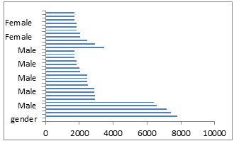
Majority of female employees works 2000 hours and below per year while men work for more than 4000 hours per year. The data portrays large significance differences between mean working hours of female and male. On average male spend more hours working per year as compared to females. The average male working hours is 3485.9 while female is 2016.5 with mean differences of over 1000 working hours. Working hours is associated with gender with female working fewer hours compared to males this may be affected by marital privilege or other commitments.  The mean working hours is higher in females as compared to males, thus gender affect working hours.

Chi-square tests of association between gender and marital status

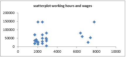
The first step in studying the relationship between two continuous variables is to draw a scatter plot of the variables to check for linearity.

We plot scatter plot with x axis being working hours and dependent variable wages.

Majority of employees work between 2000 hours and 3000 hours earning below $100000 and few work above 6000 hours though the wages is not increasing above $100000. There is no linear relationship between number one spend working per year and the amount of wages one earn. Some works less than 2000 hours in year and they earn more than 100000 dollars, while others work more than 6000 hours per year and earn less than 100000 dollars a year. Increase in working hours does no increase wage one earns and decrease in working hours does not result to a decrease in wage one earns. The two variables are not correlated with each other. The data is highly skewed to the right hand side with many extreme values. These outliers affect the average giving false picture of data. They also affect the correlation and should be check if they are real data or errors.

The Pearson moment product correlation coefficient measures the strength of association between independent and dependent variable. The Pearson moment product correlation coefficient is 0.299 which measure strength of linear association between wage earned and number of working hours in a year. The correlation coefficient is close to zero. It indicates weak linear association between working hours and wages.

Regression analysis is a statistical process for estimating the relationships among variables. It includes many techniques for modeling and analyzing several variables, when the focus is on the relationship between a dependent variable and one or more independent variables. Regression analysis helps to exclude those values that do no have significance importance in the predicting dependent variable.

Where y is wages earned and x is number of working hours per year.

R – Squared is 0.093 which means working hours only explain 9% change of respondent wages and the model is not a good fit. R – Squared is 0.093 means that when predicting a person’s total income, we will make 9% fewer errors by basing the predictions on the person’s hours of work and predicting from the regression line, as opposed to ignoring this variable and predicting the mean of income for every case.   Hours of work(X) explain 9% of the variation in income(Y) among city employees.

A slope of 1.844106 means that 1-hour increase in an employee’s amount of working hours result to an average increase in annual income of $ 1.844106. A y-intercept of 42710.94 suggests that the expected income for a person with 0 hours of work should be $ 42710.94. Moreover, from the data t= 0.488746 and p-value= 0.628968, we can conclude that the slope for hours of work is not significantly different from zero at p is greater than 0.05.

Conclusions

Descriptive and inferential data analysis was used to analyze the data on Excel 2007 software, the following were obtained. The average age of respondents is 28.66667 years with standard deviation of 1.24106, the mean wage of the respondents per year is 51200.87 with mean working hours per year of 2996.1, average number of degrees one have is 2 and on average each respondent has one kid. Gender or being male or female does not affect the marital status of the respondent. Marital status is independent of gender. There is no association between number one spend working per year and the amount of wages one earn. Increase in working hours does no increase wage one earns and decrease in working hours does not result to a decrease in wage one earns. The Pearson moment product correlation coefficient is 0.299 which measure strength of linear association between wage earned and number of working hours in a year. The correlation coefficient is close to zero. It indicates weak linear association between working hours and wages. The chi-square of association between gender and marital status produced results as follow. That gender or being male or female does not affect the marital status of the respondent. Marital status is independent of gender. The result are insignificance, the difference between the expected and observed values under null hypothesis is negligible.

References

1. Browne, C., Battista D., Geiger T., Gutknecht T. ( 2014). The Executive Opinion the Voice of the Business Community, in the Global Competitiveness. World Economic Forum, 2014, pp. 85–96.
2. Whitley E, Ball J. (2002). Statistics review 1: Presenting and summarizing data.Crit Care. 
3. Beth L. Chance, Allan J. Rossman. 2006. Mathematics.
4. Park, H., Russell, C. & Lee, J. 2007, "National culture and environmental sustainability: A cross-national analysis", Journal of Economics and Finance, vol. 31, no. 1, pp. 104-121.
5. Venkat N., Vijav V., Venu G. and Rao R. (2016). Handbook of Statistics.

      Retrieved from: https://www.sciencedirect.com/science/handbooks/01697161.

6. Joseph L. Gastwirth,Methods for Assessing the Sensitivity of Statistical Comparisons Used in Title VII Cases to Omitted Variables, 33 Jurimetrics J. 19 (1992).
7. Fisher R.A. 1925. Methods For Research Work; Macmillan Publishers: London.